
Preface
JSim's model parameter optimizers are automated tools for finding model parameter values which cause model output to best match fixed reference data. This document provides step-by-step instruction for operating the optimizers.
Prerequisites:
- Introduction to the JSim GUI (required)
- Data Files and Project Data Sets (required)
- JSim Projects (recommended)
Contents:
- Overview
- Starting the tutorial
- Understanding the model
- A Sample Optimization
- Graphs and Reports
- Stopping Criteria
- Complications
- Comments or Questions?
Overview
Suppose you wish to match output from a given model to data taken from a scientific experiment. The general process is as follows:
1) Create a data file with the experimental results and import it into the project that contains your model (see Data Files and Project Data Sets ).
2) Decide which model outputs should best match which data curves. Typically this involves a bit of exploration of model parameter space using plot pages.
3) Configure the model's "Optimizer" sub-tab with the parameters you wish to vary and the model outputs and data curves which should ideally match.
4) Push the optimizer's "Run" button and watch as the optimizer works.
5) Examine optimizer results and model outputs at new optimized parameter values.
Starting the tutorial
on your computer:
- If you have not already done so, download and install JSim on your computer.
- , the model file for this tutorial.
- , the data file for this tutorial.
- Start JSim on your computer
- Select "Import model file..." from the "Project" tab "Add" menu and load the opt1.mod model file.
- Select "Import data file..." from the "Project" tab "Add" menu and load the optdata1.tac data file.
Understanding the model
Examine the model MML to see how it works. Compile and run the model and plot the output variable named "u", which represents exponential decay. u's values are controlled by the parameters "amp" and "decay", both of which have 1 as a default value. Run the model with various values of amp and decay to get a feeling for how they affect the affect u. When you are done, restore amp and decay to their default values.
Now superimpose the curve R1s1 from the data set optdata to the plot containing u. Alter plot colors or other characteristics so that you can clearly distinguish between model output and fixed data. Now run the model varying amp and decay until you get a reasonable match between u and R1s1. This is the process the optimizer will automate. Note that both amp and decay must be altered from their defaults to get a reasonable fit. If you are confused about any of the above operations, you should probably review the documents mentioned in the introduction.
A Sample Optimization
We will now setup the optimizer to automatically perform the optimization you did "by hand" in the previous section. Restore amp and decay to their default values, and then select expon's "Optimizer" sub-tab which configures an optimization run.
The configuration is divided vertically into three sections. We'll ignore the top section for now. Look at the "Parameters to Vary" section. Here is where we will specify that amp and decay are the parameters we wish to vary. Enter "amp" (no quotes) in the Parameter column or select amp from a parameter list by clicking the down arrow button to the right of the box. The line will blacken showing the current value of amp (which should be 1) in the Start column. Fill in 0.5 and 5 in the Min and Max columns to indicate the minimum and maximum values of amp you wish to optimizer to consider. The Step column prescribes in the initial absolute (not relative) change in parameter value. For this tutorial, the default value is adequate. Once all fields in the line have contents, a check box will appear in the OK column. Optimization of this parameter may be temporarily disabled by unchecking the box. A question mark will appear in the OK column, if there is some problem with the line. Clicking on the question mark will display a message telling what the problem is.
A second (blank) line will have opened when you entered amp in the first line. Specify the parameter decay in the second line as you did amp in the first. Use the same min and max values. The "Parameters to Vary" section should now show two blackened lines, and a third blank one.
Now look at the "Data to Match" section. Here we will tell the optimizer to get the best match it can between data curve R1s1 and model output u. The first column is the dataset from which to draw the data curve. Since your project contains only a single data set (optdata), it will be automatically filled in. If you use the optimizer in projects with more than one data set, you will need to select which data set to use. In the "Curve" column enter "R1s1" no quotes or select it from the popdown list. The box should blacken. In the "Par/Expr" column, enter "u" (no quotes) or select it from the pop-down list. The first line under "Data to Match" should now be completely blackened and a check box should appear in the OK column. This checkbox (or the associated question mark) function as their counterparts in the "Parameters to Vary" section. Ignore the "Pwgt" and "Cwgt" columns for now.
The optimizer is now ready to be run. Press the "Run" button in the optimizer configuration menubar. The optimizer works by running the model for various parameter values, guessing after each run other values to try. In our case the model runs very quickly, so entire optimization run should only take a few seconds. Your plot page should now show good agreement between model output and reference data. The optimized values for amp and decay are now shown in the "Start" column of the "Parameters to Vary" section. Note that the values are good, but not perfect. Perfect values would be amp=2 and decay=3.
Graphs and Reports
The "Optimizer" sub-tab, has three sub-sub-tabs along the top margin. The "Config" (sub-sub-)tab was used to configure the optimization run. Useful results from the most recent optimization run can be viewed in the "Graph" and "Report" tabs. The "Graph" tab has seven different "View" options which should be fairly self-explanatory after you see them once. The "Report" tab should also be easy to understand. Take a few minutes to examine the graphs and report.
When using JSim versions 2.16 and above, the Optimization report now includes RMS and relative RMS (RRMS) error for individual curves when multiple, simultaneous data curve fits are run (previously, the RMS was reported for only the entire collection of curve fits). This information can be useful when data curves differ by orders of magnitude or have different dimensions. The RRMS error is calculated by taking the indivdual curve fit RMS and dividing it by the weighted standard deviation of the data curve.
RRMS error is only reported on non-negative data.
One part of the report, that can be difficult to understand, is the "Condition number" which gives you an idea about how useful the confidence intervals for the given optimization are. Please see JSim Optimization Report: Condition Number for more details. Note that since we did no relative data weighting, the weighted and unweighted residual graphs are identical and the "Point weigths" graph contains nothing useful.
All three Optimizer sub-tabs possess a "Run" button in the menubar. The results of the optimizer will be same in each case. What will vary will be the reporting the user receives as the optimizer works. Currently JSim does not support the user switching between different types of feedback while the optimizer is running.
Stopping Criteria
Return now to the optimizer's "Config" tab. The top third, labelled "Model Optimizer Configuration" controls the optimization algorithm to be used, and the parameters controlling when the optimizater stops work. The optimizer almost never gets a perfect match between data and model output. Therefore, stopping criteria are provided to tell it when it has done a "good enough" job.
Some stopping criteria are common to all algorithms, while some are algorithm-specific. Common stopping criteria are described below. See JSim Optimization Algorithms for algorithm-specific details.
The common stopping criteria are:
- Max # runs: The optimizer will stop if it has run the model this many times.
- Min RMS error: The optimizer will stop if the mean RMS error between reference data and model output is less than this value. The RMS error is calculated as
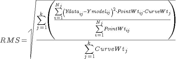
where there are j=1 to k curves, each curve having a curve weight, CurveWeightj, and having i=1 to Nj data points, Ymodelij, and corresponding point weights, PointWtij.
- Min par step: The optimizer will stop if it is considering parameter values that vary less than this value.
If unrealistic values for the stopping criteria are specified, the model optimizer may either run forever, or stop before any useful work is done. You always have the option of cancelling a long optimization run, and the best values so far calculated will be retained.
Complications
Real world models and data will not fit so easily as in this idealized example. This introduction serves only to show how to operate the JSim optimizer, but does attempt to address the large scientific problem of how best to optimize parameters to reference data. Future tutorials will address these issues. Some complicating factors are:
- Errors in mathematical formulation of models which no mere parameter adjustments can hope to compensate for.
- Noisy data may good fits difficult. Models may be expected to fit multiple data curve. Relative weighting of RMS error between data points or data curves may be highly subjective.
- Optimizer algorithms generally perform more and more poorly the larger the number of varying parameters.
Comments or Questions?
Model development and archiving support at https://www.imagwiki.nibib.nih.gov/physiome provided by the following grants: NIH U01HL122199 Analyzing the Cardiac Power Grid, 09/15/2015 - 05/31/2020, NIH/NIBIB BE08407 Software Integration, JSim and SBW 6/1/09-5/31/13; NIH/NHLBI T15 HL88516-01 Modeling for Heart, Lung and Blood: From Cell to Organ, 4/1/07-3/31/11; NSF BES-0506477 Adaptive Multi-Scale Model Simulation, 8/15/05-7/31/08; NIH/NHLBI R01 HL073598 Core 3: 3D Imaging and Computer Modeling of the Respiratory Tract, 9/1/04-8/31/09; as well as prior support from NIH/NCRR P41 RR01243 Simulation Resource in Circulatory Mass Transport and Exchange, 12/1/1980-11/30/01 and NIH/NIBIB R01 EB001973 JSim: A Simulation Analysis Platform, 3/1/02-2/28/07.