
Michaelis-Menten Reaction Sequence for solutes A to E in a stirred tank flowing reactor with constant volume, Vol, and step jumps in flow and in reaction rates. This is the second in a series of four models to account for substrate capacitance in enzymatic networks. The first model is Linear.Reaction.Sequence (Model #0423).
Description
 A reaction sequence A-->B-->C-->D-->E can be represented many ways to approximate the biological
 form of the reactions. This version is the next to simplest: Michaelis-Menten unidirectional reaction
 clearances, giving progress curves as in a bioreactor, but with additional factor of a flow through
 the mixing chamber. The flow term is first order for all solutes in the sequence, but the reaction
 terms are saturable MM, Vmax*A/(Km+A).
     The inflowing initial solute A, the flow, ml/sec, Flow*CinA, equals the sum of the outflow
 clearance plus the last reaction E--> ?, i.e.  G*E, then the outflow concentration of A in the
 steady state goes to 50% of CinA (Do this by setting Flow1 = Flow2 = 0.05 ml/sec and setting GA1
 and GA2 also to 0.05 and run the program. The other reaction rates, to form C, D, and E are set
 identical to that to form B from A, the result is that steady state concentrations for A, B, etc
 go to 0.5, 0.25, 0.125, 0.0625, and 0.03125, all at one half of its predecessor.
     This program illustrates the transient delays between steady state, and the form of the transients.
 With MM kinetics there is really no enzyme there, and no binding of the reactants in the process of
 the reaction. All of the delay is due to the combination of flow and the reaction, exactly similar
 to the first order reaction kinetic model (Model #423). The initial conditions are zero for all solutes
 so the time constant for the initial entry would be simply the volume divided by flow, Vol/Flow1,
 in seconds, if there were no reaction. The reaction, augmenting the disappearance of A, shortens the
 time constant so that it is Vol/(GA + Flow1).
      The second transient is due to a step increase (or decrease) in flow at time TFjump (at t=30 s
 with this parameters set (MMpure.181026.Km). The third transient is a step change in the reaction
 rates at time TGjump. The Verification Process is the same as for the linear kinetics, and which does
 verify the code when the solute concentrations are 1 mM when the KmA was 21.416 mM.
      The solution to the differential equation for solute A is accomplished using the numerical solvers,
 but it is also solvable analytically. The three transients, at t = 0, t= 30 s and t=60 s, are expressed
 in three analytical equations. Their sum fits exactly the numerical solutions to the systems equations.
 VERIFICATION! Try this out using the difference ODE solvers: it turns out the DOPRIS5 (an advanced
 RungeKutta algorithm) gives a more precise fit to the analytical solution than either of the more
 powerful stiff solvers, CVODE or Radau. At the steep parts of the transients DOPRIS5 is still good
 to 7 decimal digits, while the other supposedly superior solvers, CVODE and Radau are good only 5 or
 6 decimal digits. In the steady state they all give the same correct answers.
       For solutes B through E, the analytical solutions are more complex, and have not been developed.
 For these it is much faster to use the numerical solutions to the ODEs; the analytical solutions for
 solute E would be, because of their complexity, much slower to compute, and maybe not even as accurate
 as the numerical solutions, even for this rather simple model system. What we know is that the steady
 state solution match exactly to the predicted steady state values for A through E.
       The basis for this series of models to account for substrate capacitance in enzymatic networks is
 the model Linear.Reaction.Sequence (Model 0423); this one is the second: MM.Reaction.Sequence.
 The third, MM.Lag.React.Seq (Model 0425) adds a lag to each reaction to account for capacitance.
 The fourth, Enzyme.React.Seq.Full.Kinetics (Model 0426) accounts for enzyme binding kinetics as well.
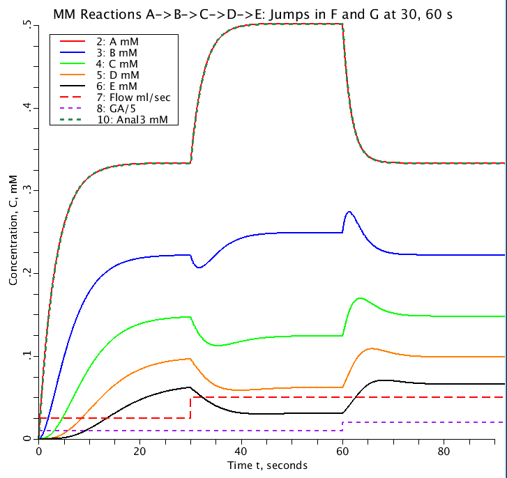
Figure: Progress curves for a sequence of reactions from substrate A to E in a compartment with flow through the compartment. All substrates have initial concentration of zero with A in (CinA) set to 1 mM. Flow doubles from 0.025 to 0.05 ml/sec at t= 30 sec. Consumption (the flow of fluid cleared of substrate per unit time) doubles from 0.05 to 0.1 ml/sec at t= 60 sec. GA is the consumption of substrate A and Anal3 is the analytical solution for substrate concentration A as a function of time.
Equations
The equations for this model may be viewed by running the JSim model applet and clicking on the Source tab at the bottom left of JSim's Run Time graphical user interface. The equations are written in JSim's Mathematical Modeling Language (MML). See the Introduction to MML and the MML Reference Manual. Additional documentation for MML can be found by using the search option at the Physiome home page.
- Download JSim model MML code (text):
- Download translated SBML version of model (if available):
We welcome comments and feedback for this model. Please use the button below to send comments:
 Easterby, JS. A generalized theory of the transition time for sequential enzyme reactions.
    Biochem J. 199: 155-161, 1981.

 Cascante M, Melendez-Hevia E, Kholodenko B, Sicilia J, and Kacser H. Control analyis
   of transit time for free and enzyme-bound metabolites: physiological and
   evolutionary significance of metabolic response times. Biochem J 308: 895-899, 1995.

 Bassingthwaighte JB. Capacitance in metabolic netowrks. 2019 (in prep for submission to Biophys J)
Please cite https://www.imagwiki.nibib.nih.gov/physiome in any publication for which this software is used and send one reprint to the address given below:
The National Simulation Resource, Director J. B. Bassingthwaighte, Department of Bioengineering, University of Washington, Seattle WA 98195-5061.
Model development and archiving support at https://www.imagwiki.nibib.nih.gov/physiome provided by the following grants: NIH U01HL122199 Analyzing the Cardiac Power Grid, 09/15/2015 - 05/31/2020, NIH/NIBIB BE08407 Software Integration, JSim and SBW 6/1/09-5/31/13; NIH/NHLBI T15 HL88516-01 Modeling for Heart, Lung and Blood: From Cell to Organ, 4/1/07-3/31/11; NSF BES-0506477 Adaptive Multi-Scale Model Simulation, 8/15/05-7/31/08; NIH/NHLBI R01 HL073598 Core 3: 3D Imaging and Computer Modeling of the Respiratory Tract, 9/1/04-8/31/09; as well as prior support from NIH/NCRR P41 RR01243 Simulation Resource in Circulatory Mass Transport and Exchange, 12/1/1980-11/30/01 and NIH/NIBIB R01 EB001973 JSim: A Simulation Analysis Platform, 3/1/02-2/28/07.