
One program generates noisy data and another program calculates the linear regression using the Y fractional error.
Description
(Run the GenerateNoisyData model first. Directions at end of this
explanation. Then run LOOPS with the LinearRegression model. )
There are several different methods for calculating a linear regression:
(1) the standard Y-on-X regression minimizing the vertical distance to
the regression line (assumes all the error is in Y);
(2) the X-on-Y regression minimizing the horizontal distance to the
regression line (assumes all the error is in X);
(3) the angle bisector of the Y-on-X and X-on-Y regression line, splitting
the difference between the Y-on-X and the X-on-Y regressions.
(4) the orthogonal distance regression minimizing the perpendicular distance
between the data and the regression line (assumes equal error in X and Y);
and
(5) the geometric mean regression, assumes a ratio of error between the y
data and the x data.
All of these methods can be reduced to a single method.
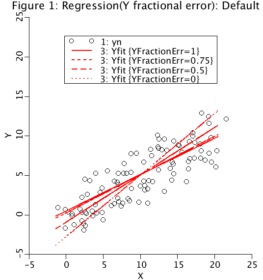
The Y fractional error, YFE is error in the Y data divided by the sum of the
error in the Y and X data.
YFE = 1.0 for Y-on-X regression.
YFE = 0.75 for 75% of the error in Y and 25% of the error in X.
YFE = 0.5 for equal error in both Y and X.
YFE = 0.0 for X-on-Y regression.
YFE can range between 0 and 1 for geometric mean regression.
If the Y data was velocity and the x value was distance, YFE =0 or 1 makes
sense. However, for other values of YFE, it is difficult to say what the
meaning is of a measure which combines the square root of velocity-squared
plus distance-squared.
This leads us to proposing that in a linear regression the data should be
normalized by first subtracting the mean and then dividing by the standard
deviation. The regression for data which has been non-dimensionalized is
y=+x or y=-x,
depending on the sign of the correlation coefficient. Redimensionalize the data
yields
Y - ybar R (X - xbar)
-------- = ------------
sigmaY sigmaX
where R is given by
/ YFE - 0.5 \
|----------------|
| 2 |
\YFE - YFE + 0.5/
R = SIGN(1.0, rcor) ABS(rcor) .
For Y-on-X, R=rcor. For X-on-Y, R=1/rcor. For orthogonal distance regression,
R=sign(rcor).
When this routine is used to compute an orthogonal distance regression,
what is computed is the orthogonal distance minimization for the data
non-dimensionalized and normalized to have mean zero and variance 1.
This minimum does not correspond to the actual minimum when the data is
redimensionalized back to its original values. When the X and Y data
have different units, this is preferable, because the orthogonal distance
of a mixed metric is undefined.
The optimizer has been set up to produce either the Y-on-X regression
(fitting the noisy yn as a function of x) or the the X-on-Y regression,
(fitting the noisy xn as a function of y).
For generating the noisy data, use the GenerateNoisyData model.
To generate noisy data do the following steps:
(1) Delete the Data File, "Noisy"
(2) Set n.max to the number of points to generate.
(3) set xslope and yslope. The original data will run from
xslope*n.min<=x<=xslope*n.max and
yslope*n.min<-y<=yslope*n.nax. The expected value of
the slope of the regression is SLOPE= yslope/xslope,
when xslope not equal to zero.
(4) Set xstdev, and ystdev, the standard deviation of the
added noise. NOTA BENE, the calculated standard deviations
of x and y will equal the standard deviations of the
x and y noise only if the slopes are set to zero.
(5) Store project data set (see File button on plot page)
under name as Noisy.
(6) User has CHOICE of uniform (-1 to 1) or Gaussian noise
To verify that the x- and y-data is either Gaussian or uniform, set
xslope and yslope to zero in the Run Time menu and compare xstdev
with xsd, and ystdev with ysd.
Equations
None.
The equations for this model may be viewed by running the JSim model applet and clicking on the Source tab at the bottom left of JSim's Run Time graphical user interface. The equations are written in JSim's Mathematical Modeling Language (MML). See the Introduction to MML and the MML Reference Manual. Additional documentation for MML can be found by using the search option at the Physiome home page.
- Download JSim model MML code (text):
- Download translated SBML version of model (if available):
We welcome comments and feedback for this model. Please use the button below to send comments:
None
Please cite https://www.imagwiki.nibib.nih.gov/physiome in any publication for which this software is used and send one reprint to the address given below:
The National Simulation Resource, Director J. B. Bassingthwaighte, Department of Bioengineering, University of Washington, Seattle WA 98195-5061.
Model development and archiving support at https://www.imagwiki.nibib.nih.gov/physiome provided by the following grants: NIH U01HL122199 Analyzing the Cardiac Power Grid, 09/15/2015 - 05/31/2020, NIH/NIBIB BE08407 Software Integration, JSim and SBW 6/1/09-5/31/13; NIH/NHLBI T15 HL88516-01 Modeling for Heart, Lung and Blood: From Cell to Organ, 4/1/07-3/31/11; NSF BES-0506477 Adaptive Multi-Scale Model Simulation, 8/15/05-7/31/08; NIH/NHLBI R01 HL073598 Core 3: 3D Imaging and Computer Modeling of the Respiratory Tract, 9/1/04-8/31/09; as well as prior support from NIH/NCRR P41 RR01243 Simulation Resource in Circulatory Mass Transport and Exchange, 12/1/1980-11/30/01 and NIH/NIBIB R01 EB001973 JSim: A Simulation Analysis Platform, 3/1/02-2/28/07.