Fitting an equation for a quadratic with added noise is used to illustrate the MonteCarlo Graphical User Interface.

Description

A quadratic curve, Quad(t), is generated. 10% proportional noise
using the seed 12345 (in Solver GUI), is added producing NoiseQuad(t).
The noisy curve, NoiseQuad, and the non-noisy curve, Quad, are saved using
the "Store data set" from the pull down menu under the File Tab on the
Figure 1 Plotpage. This data is saved as Fig1Save.

The data stored in Fig1Save is plotted again in Figure 2 
(red for NoiseQuad, Black for Quad.) Quad (from the
Monte Carlo model is plotted in green dashes. The optimizer is
run to get the best fit for a0, a1, and a2. This moves the 
dash green line (Quad, MonteCarlo) slightly off the black
line (Quad from Fig1Save).

Now we turn off (show button unchecked) the saved data, curves
1 and 2. Use "Store data set" to save the optimized Quad curve
(curve 3, dashed line), naming the data set BestFit.

For the MonteCarlo simulation, we are going to add noise to this
best fit curve many times, and optimize these new noisy data sets.

The optimization GUI should contain
 
Data Set	Curve		Par/Expr	Pwgt	Cwgt	OK   
Fig1Save	NoisyQuad	Quad		1	1	CheckMark

This needs to be reset to
Data Set	Curve		Par/Expr	Pwgt	Cwgt	OK
Fig1Save	NoisyQuad	Quad		1	1	blank
BestFit		Quad		Quad		1	1	CheckMark

NOW GO TO THE MonteCarlo GUI. Set the following parameters

# optimizations: 1000
random seed: 6789
distribution: gaussian
magnitude 0.1;
add method:proportional.

The "add methods" are called "proportional" and "additive". 

"proportional" noise
NewValue=OldValue*(1+fraction*Noise)  where Noise has mean 0 and variance 1
                                      and 0<=fraction<0.25.
"additive" noise
NewValue = OldValue+amplitude*Noise   where Noise has mean 0 and variance 1.

Run the MonteCarlo simulation.

There are a wide range of data items that the user can access. Starting with
Reports, there are  two views: Summary and Detail. Summary summarizes all
1000 runs. Detail gives the particular details of an individual run.

From the summary run we have
Parameter statistics:
  parameter     mean         sd     
     a0         1.026       .0521   
     a1         .772        .321    
     a2         1.231       .3582   

Normalized Covariance Matrix:
                 a0          a1          a2     
     a0           1        -0.8481      .7424   
     a1        -0.8481        1        -0.9665  
     a2         .7424      -0.9665        1     

Parameter estimates:
  opt#       a0          a1          a2         
...
  646      .9243       1.792      -0.0359 
...
  881      1.192      -0.3187      2.558   
...
Graphically, we can view Summary Plots of histograms of a0, a1, and a2,
and two parameter scatter plots a0 with a1, a0 with a2, and a1 with a2.

Using the detail view, we have access to any of the 1000 individual runs.
Using the histogram plot for a2, we locate the max and min values for a2
and view the associated runs, 881 and 646 respectively.

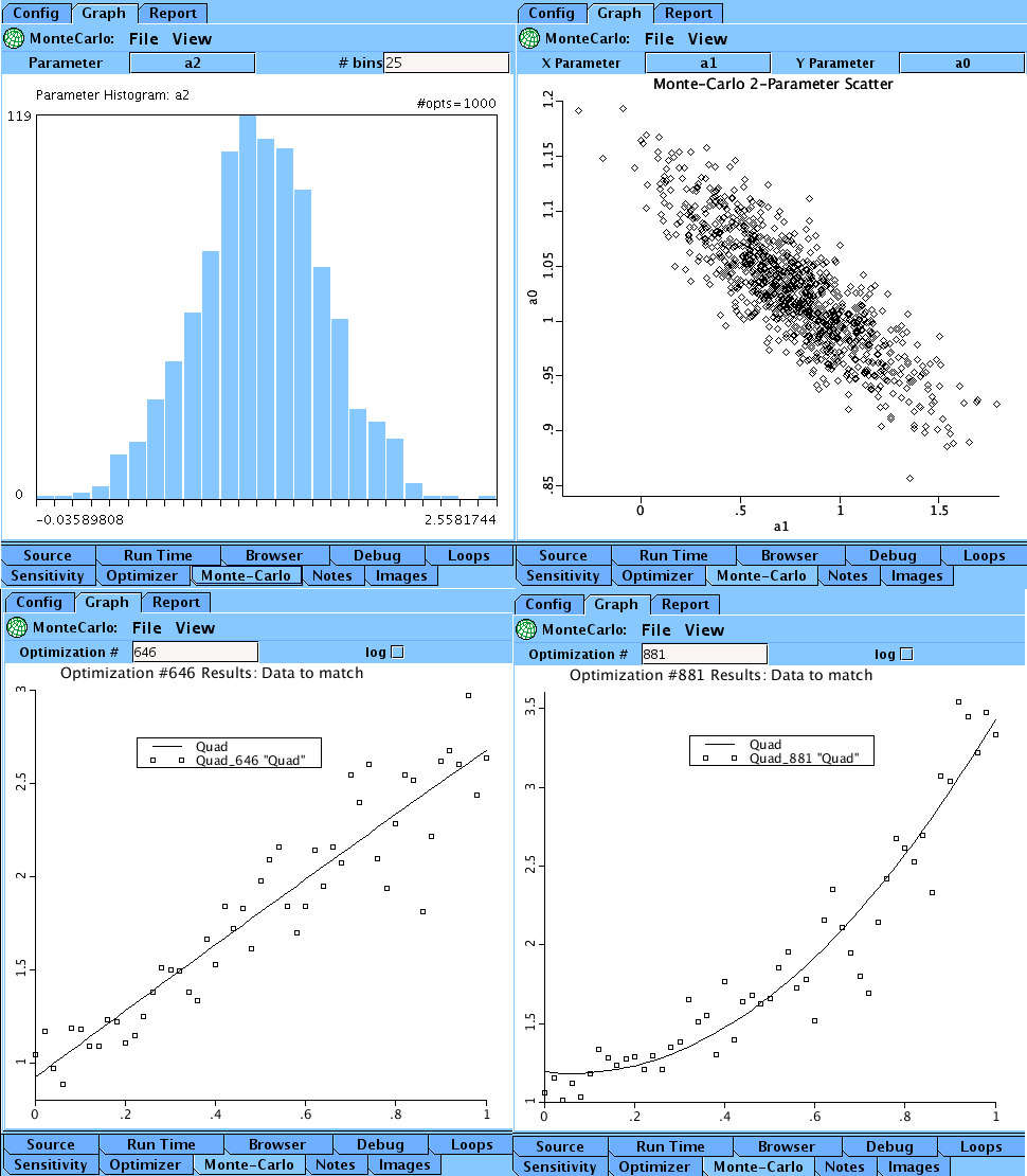
Upper Left: The histogram for parameter a. Upper Right: The scatter plot for parameters b and c.
Lower Left: The optimized curve and data for run 646. Lower Right: The optimized curve and data for run 881.

Equations

None.

The equations for this model may be viewed by running the JSim model applet and clicking on the Source tab at the bottom left of JSim's Run Time graphical user interface. The equations are written in JSim's Mathematical Modeling Language (MML). See the Introduction to MML and the MML Reference Manual. Additional documentation for MML can be found by using the search option at the Physiome home page.