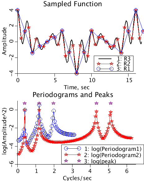
A continuous function, a sum of 4 cosines, is sampled at delta-t =1/2 and undersampled at delta-t=1 illustrating the folding of frequencies around the Nyquist frequency.

Description

The Fourier transform of an undersampled continuous function "folds"
higher frequencies into lower frequencies. 

Let series be of length N, and the series samples (V(i), i=1..N), sampled at  
(t(i), i=1..N). The intervals between consecutive samples is t.delta. The model is
initialized with an odd number of samples. t.min=t(1). t.delta is the
interval between samples. t.ct, the number of samples, equals N.

The maximum number of frequencies is
kmax = N/2, N even,
     = (N-1)/2, N odd.
The frequencies are f(i) = i/(N*t.delta), i=1..kmax.
The highest frequency is 1/(2*t.delta) which is called the Nyquist frequency,
also called the folding frequency. In radians/sec it is 2*PI/(2*t.delta).

Let 
odd=0 , N is even and
odd=1, N is odd.

The forward transform is calculated as
      N
A0 = Sum(V(i)/N).
     i=1

for j=1 to kmax, 
   IF ( j not equal to kmax+odd),
                N
      A(j)=2/N*sum(V(i)*cos(2*PI*f(j)*(t(i)-t.min-t.delta)) 
               i=1

                N
      B(j)=2/N*sum(V(i)*sin(2*PI*f(j)*(t(i)-t.min-t.delta)) 
               i=1
   ELSE
            N
      A(j)=sum( (-1)^(round((t(i)-t.min)/t.delta)-1)*V(i)/N).
           i-1

      B(j)=0.
   END   
END

The Periodogram estimate P(j) = A(j)*A(j)+B(j)*B(j).

The back transform is given as
for i = 1 to N

        kmax
V(i)=A0+sum ( A(j)*cos(2*PI*f(j)*(t(i)-t.min-t.delta)) + B(j)*sin(2*PI*f(j)*(t(i)-t.min-t.delta)) )
        j=1

The original series was built using four frequencies,
[ PI/8, 3PI/8, 11PI/8 and 13PI/8 radians] and unit amplitudes.
The periodograms (lower plot) are plotted in blue for R1 (under sampled)
and R2 (adequately sampled).

R2 with a deltaT=1/2 has a cut off frequency of 2*PI radians, and hence
the periodogram for R2 captures this information.

R1 with a deltaT=1 has a cut of frequency of PI radians. Therefore
the last frequency of 13PI/8 is folded to PI-(13PI/8-PI) = 3PI/8 and the 
peak for the periodogram is boosted from 1 to 4 (1+1)^2=4. The peak
that was at 11PI/8 appears as a new peak at PI-(11PI/8)-PI) = 5PI/8.
Notice how the peaks are folded around the Nyquist frequency. The
decaying envelope around each frequency peak is because the frequencies
calculated do not match the frequencies used in the function. By shifting
the starting times of the samples (Parameter set Sharp) we can make the
peaks appear at the exact frequencies.

Upper Panel: A time series of Gaussianly distributed random numbers with mean=0, variance=4.
Lower Panel: The autocovariance function (black) and the autocorrelation function (red) are plotted as functions of the lag.

Equations

See Description above.

The equations for this model may be viewed by running the JSim model applet and clicking on the Source tab at the bottom left of JSim's Run Time graphical user interface. The equations are written in JSim's Mathematical Modeling Language (MML). See the Introduction to MML and the MML Reference Manual. Additional documentation for MML can be found by using the search option at the Physiome home page.