A rational exponential function, R(x)= exp(-P(x)/Q(x)), where P and Q are polynomial in x expressed p1 + p2*x + p3*x^2 +.. pn*x^(n-1) and 1 + q1*x + q2*x^2 + ....+ qn*x^m, where n is not necessarily = m.

Description

 A rational exponential function, R(x) = exp(-P(x)/Q(x)), 
 where P and Q are polynomial in x expressed p1 + p2*x + p3*x^2 +.. pn*x^(n-1)
 and 1 + q1*x + q2*x^2 + ....+ qn*x^m, where n is not necessarily = m.

 Such functions are good generalities for monotonic decay curves for many situations: 
 washout curves, isotopic decays (not alway exponential), pharmacokinetics, or things 
 rising to a plateau from zero, fitted with F(x) = 1-R(x).
 
 This is a general kind of decay function, the basic form being a single 
 exponential decay. It can be expanded as desired by adding more terms to P and Q.
 With just up to the cubic, the adjustment to the parameters can steepen or make 
 shallower the inital decay while keeping the tail long. 

 Consider the TEST (T) curve the standard curve. Note that the Parameter file, 
 'ConstRloop', run using the 'Loops' page, scales through sets of parameters all 
 giving the same R curve. With each loop, 1 is added to p1 through p3 and to q0 
 through q2, but not q3. Explain why this works.

 Reducing the curvature: Increasing q2 and q3 does this; increasing q1 causes
 slowing of the early downslope but does little to the tail; increasing q2 
 delays the middle and the tail but not the early downslope.
 
 Increasing the curvature: Increase p1, p2 or p3; put more weight on p3 to bring the
 tail down sooner; put weight on p1 and p2 make the initial downslope faster.

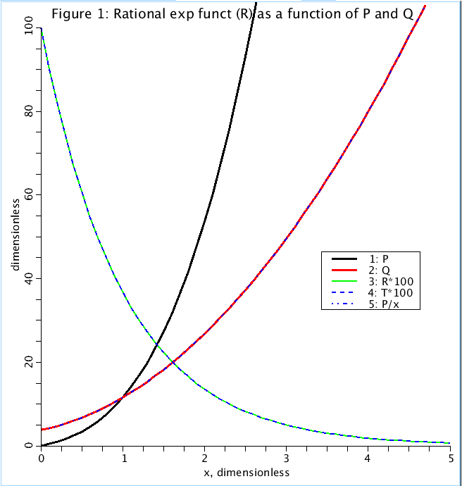
Figure: Rational exponential (R) and four term polynomials P and Q, which make it up, are plotted as a function of x. T is the test exponential of form exp(-x). The coefficients of P and Q are picked so that R fits T.

Equations

The equations for this model may be viewed by running the JSim model applet and clicking on the Source tab at the bottom left of JSim's Run Time graphical user interface. The equations are written in JSim's Mathematical Modeling Language (MML). See the Introduction to MML and the MML Reference Manual. Additional documentation for MML can be found by using the search option at the Physiome home page.