Simple low pass, high pass, and bandpass filters are illustrated by four examples.

Description

This program convolves low pass and high pass filters with a time series
of Gaussian white noise. The ends of the series are "wrapped." 

An example will clarify this.
Let A3 be the filter (1/3, 1/3, 1/3). We will convolve it with series
Y=(y0, y1,y2,y3,y4,y5):
A3(t) convolved with Y(t)=H(t) =[ (y5+y0+y1)/3, (y0+y1+y2)/3, ... (y4+y5+y0)/3 ]. 
Note how y5 and y0 are wrapped. It is as if the series was
[y5, y0, y1, y2, y3, y4, y5, y0].

A high pass filter can be generated by differencing adjacent points.

By combining low and high pass filters, bandpass filters can be constructed.
Filtering operations can introduce phase shifts in the estimated Fourier
coefficients.

A Fourier transform of a time series is a least squares fit of the
time series with a set of sine and cosine functions. Since the chosen
frequencies used in the transform are orthogonal functions, their coefficients
can be found indpendently.

The periodogram at a give frequency is constructed by adding the squares
of the Fourier coefficients, i.e.,

P(f)=A(f)*A(f)+B(f)*B(f).

This is called a Power Spectrum and is usually plotted log(P) vs. log(f).
It is important to note that the Power Spectrum is not the spectrum of
the time series. It is a biased estimate of the spectrum.
The Fourier transform can be used to compute the periodogram of the 
original series, P1, and the filtered series, P2. The ratio P2/P1
is the periodogram of the Filter.

In Example 1, a series of 365 Gaussian random numbers has been
generated and low passed with a 7 point low pass filter. It should be noted
that although the periodograms of the time series before and after
filtering are noisy, the frequency response of the filter is smooth.

In Example 2, the same series is low passed twice with the 7 point
filter. Note that the Frequency response of the Filter appears to be
the same, but notice the scaling of the amplitude--it doubles.

In Example 3, the same series is high passed with a two point difference
filter.

In Example 4, the same series is band passed.

These are simple examples and more complex kinds of filters have been
designed.

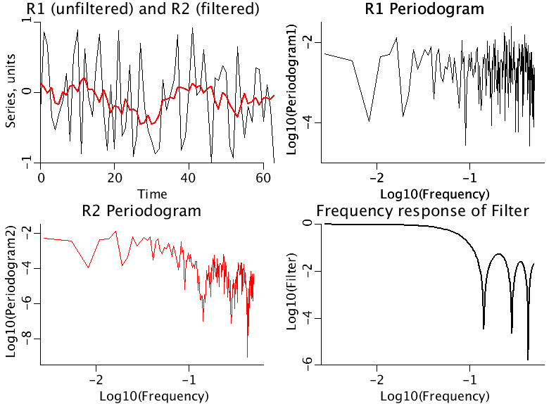
The four panels illustrate a low-pass filter.
Upper Left: The first 60 points of a 365 point series are plotted (black). A seven point running average is applied, and the result is plotted in red.
Upper Right: The periodogram of the original series is plotted log-log.
Lower Left: The periodogram of the series after filtering is plotted log-log.
Lower Right: The ratio of the two periodograms is plotted log-log showing the frequency response of the seven point running average filter.

Equations

See Description above.

The equations for this model may be viewed by running the JSim model applet and clicking on the Source tab at the bottom left of JSim's Run Time graphical user interface. The equations are written in JSim's Mathematical Modeling Language (MML). See the Introduction to MML and the MML Reference Manual. Additional documentation for MML can be found by using the search option at the Physiome home page.