Table of Contents

1. Introduction

2. Methods using a simple two-region model

3. Examples using the two-region model

1. Introduction

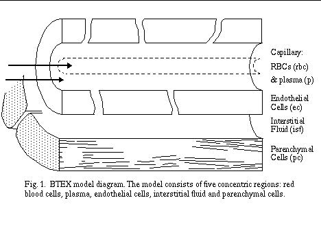
A typical blood-tissue exchange (BTEX) unit is shown in Fig. 1. There are five concentric regions and two of them are flowing regions (RBC and plasma). The two major assumptions in our BTEX model are:

(1) plug flow for RBC and plasma;

(2) instantaneous mixing in the radial direction within one region; but not in the axial direction.

So this is a axially-distributed model governed by five partial differential equations (PDE) for one chemical species (one PDE for one region). In analogy to compartmental model, this axially distributed model becomes a five-compartment model governed by ordinary differential equations (ODE) when the axial diffusion can be considered instantaneous.

2. Methods using a simple two-region model

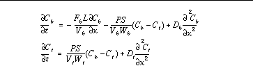
For simplification, let's consider the vascular space (RBC and plasma) as the blood region and the extravascular space (endothelial cells, interstitium and parenchymal cells) as the tissue region. The model in Fig. 1 is then reduced to a two-region model or two one-dimensional PDE models (Fig. 2).

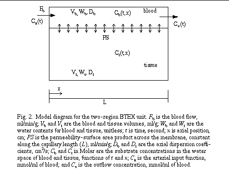
The governing eqations are

with boundary conditions:

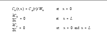
For calculation of the outflow concentration, C_v ( t ) = C_b( t,x ) W_b at x = L .

We use time-split method to solve the set of PDE's. The length of the capillary-tissue unit is divided into N_seg segments. The key of the time-split method is to use the matching time and spatial step. The mean transit time for the fluid that never leaves the vascular space is V_b / F_b . So if the numeric time step is the mean transit time divided by the number of segments,

then for each time step each fluid element will slide downstream by exactly one segment.

The time-split method is carried out in the following sequence for each time step:

(1) sliding at the beginning of the time step;

(2) exchange between the two regions for each pair of blood and tissue segments; the model equations become a set of ODE's;

(3) axial diffusion for each region.

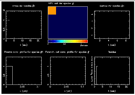
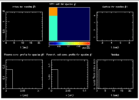
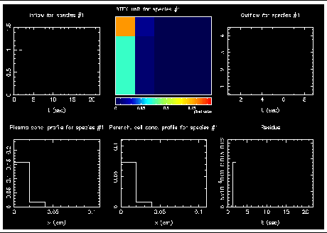
The time-split method is illustrated in the following figures. The model parameters are F_b = 1 ml/min/g, V_b = 0.07 ml/g, V_t = 0.71 ml/g, W_b = W_t = 1, PS = 3 ml/g, and D_b = D_t = 0.00005 cm²/s, N_seg = 5, C_b( t,x ) = C_t( t,x ) = 0 at t = 0, and C_a( t ) is a pulse function with duration of one numeric time step. Each figure has one color image five X-Y plots. The color image (middle panel of the top row) shows the substrate concentrations in the BTEX unit. The color code represents the concentration level. The concentration profiles along the capillary length are also shown in the two left panels at the bottom. The input function (top left), outflow function (top right) and the residue function (bottom right) are time series.

(1) Sliding at the beginning of a time step. The substrate appeared in the first segment of blood.

(2) Exchange for the time step. The substrate appeared in the first segment of the tissue region due to exchange.

(3) Axial diffusion for the time step. The substrate spread out in the axial direction due to axial diffusion.

3. Examples using the two-region model

Animation is used to show the following examples. Click on either Animated GIF or MPEG movie.

(a) No exchange, i.e., PS=0; No axial diffusion, i.e., D=0

btex10_anim_0.gif69.02 KB

 

(b) No exchange, i.e., PS=0; Axial diffusion coefficient D=0.00005 cm²/s

(c) PS=3 ml/min/g; Axial diffusion coefficient D=0.00005 cm²/s

N_seg = 5

btex20_D_anim_0.gif6.84 KB

N_seg = 30

btex20_D_anim_1.gif85.52 KB