
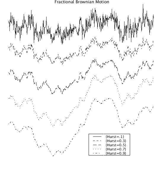
Generate both fractional Gaussian noise (fGn) and fractional Brownian motion (fBm) series using the Davies-Harte algorithm.
Description
The Davies-Harte algorithm is used to generate fractional Gaussian noise (fGn) and
fractional Brownian Motion (fBm). The sequences can be saved for processing with the
other fractal programs.

The Davies-Harte algorithm is realized here with out resorting to complex
quantities:

Let the autocorrelation sequence for fGn be given as

s(n) = (  |n+1|^2H - 2|n|^2H +|n-1|^2H  ) * var/2, where

n=0,1, ... N, 2H is twice the Hurst coefficient and var is the variance.

Define
r(n)=(  |N-n+1|^2H-2*|N-n)^H2 +|N-n-1|^H2  )*(var/2) and
and

S(n2) = if(n2<=N) s(n2) else r(n2-N) for n2 = 0 ... 2N-1.

Create C1 from S using the discrete Fourier cosine transform:

                              2 N - 1
                               -----
                                \               n2 k PI
                      C1(k) =    )    S(n2) cos(-------)
                                /                  N
                               -----
                              n2 = 0

Let Vr and Vi be defined by
when(n2=n2.min)			{Vr= randomg()*sqrt(C1(0)*2*N);
                		 Vi=0;				}
event( (1<=n2) and (n2<N) )	{Vr=randomg()*sqrt(C1(n2)*N);
                                 Vi=randomg()*sqrt(C1(n2)*N);	}
event( N=n2) 			{Vr=randomg()*sqrt(C1(N)*2*N);
                    		 Vi=0; 				}
event( (N<n2) and (n2<=n2.max) ) {Vr = Vr(n2.max+1-n2);
                                  Vi =-Vi(n2.max+1-n2); 	}
where randomg() is a Gaussian distributed random number with mean 0
and variance 1.

Define fgp as
             /2 N - 1                    \   /2 N - 1                    \
             | -----                     |   | -----                     |
             |  \                n2 k PI |   |  \                n2 k PI |
    fgp(k) = |   )    Vr(n2) cos(-------)| + |   )    Vi(n2) sin(-------)|
             |  /                   N    |   |  /                   N    |
             | -----                     |   | -----                     |
             \n2 = 0                     /   \n2 = 0                     /

for k=0 to N.

    fGn(m) = fgp(m), for m=0 to N.

The relationship between fBm and fGn is given by

                                         m
                                      -----
                                       \
                             fBm(m) =   )   fGn(j),  for m=0 to N.
                                       /
                                      -----
                                      j = 0


The spectra for fGn is given by

SfGn=A/j^(2*Hurst-1) and for
fBm as
SfBm= B/j^(2*Hurst+1) where j is the frequency.

The periodograms of fGn and fBm are calculated. The fGn series is
sorted and used to calculate the cumulative Gaussian distribution.

CAVEAT: Model is slow for N >2,000 as the Fourier transforms used
       here are not the complex Fast Fourier Transforms. The code utilizes
       discrete cosine and sine transforms and treats all quantities as
       real variables because JSim does not support complex variables and
       the FFT cannot be written as a single simple equation.
Equations
None.
The equations for this model may be viewed by running the JSim model applet and clicking on the Source tab at the bottom left of JSim's Run Time graphical user interface. The equations are written in JSim's Mathematical Modeling Language (MML). See the Introduction to MML and the MML Reference Manual. Additional documentation for MML can be found by using the search option at the Physiome home page.
- Download JSim model MML code (text):
- Download translated SBML version of model (if available):
- No SBML translation currently available.
- Information on SBML conversion in JSim
We welcome comments and feedback for this model. Please use the button below to send comments:
Please cite https://www.imagwiki.nibib.nih.gov/physiome in any publication for which this software is used and send one reprint to the address given below:
The National Simulation Resource, Director J. B. Bassingthwaighte, Department of Bioengineering, University of Washington, Seattle WA 98195-5061.
Model development and archiving support at https://www.imagwiki.nibib.nih.gov/physiome provided by the following grants: NIH U01HL122199 Analyzing the Cardiac Power Grid, 09/15/2015 - 05/31/2020, NIH/NIBIB BE08407 Software Integration, JSim and SBW 6/1/09-5/31/13; NIH/NHLBI T15 HL88516-01 Modeling for Heart, Lung and Blood: From Cell to Organ, 4/1/07-3/31/11; NSF BES-0506477 Adaptive Multi-Scale Model Simulation, 8/15/05-7/31/08; NIH/NHLBI R01 HL073598 Core 3: 3D Imaging and Computer Modeling of the Respiratory Tract, 9/1/04-8/31/09; as well as prior support from NIH/NCRR P41 RR01243 Simulation Resource in Circulatory Mass Transport and Exchange, 12/1/1980-11/30/01 and NIH/NIBIB R01 EB001973 JSim: A Simulation Analysis Platform, 3/1/02-2/28/07.