This model simulates the diffusion of a substance through a region with a constant diffusivity and different solubilities inside and outside the region.

Description

One dimensional diffusion into and across a uniform slab in which the solubility in the slab is different from that in the solutions outside. The slab partition coefficient, Lambda, = the ratio of inside/outside concentrations at equilibrium. Solubility in the two solutions is the same, in this case. On each side of the region the concentration is fixed at C_lh = 10 mM and C_rh = 3 mM. Initially the concentration in the prescribed region is 0 mM. Diffusion begins at t = 0 seconds and progresses according to the governing equation for diffusion in one dimension with a constant D given below.

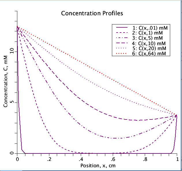
Figure: Axial profiles of concentration, C, at differing time intervals ( t= 0.1, 1, 5, 10, 20, 64 sec)
showing diffusion along axis. Concentration on left hand side (C_lh) = 10 mM and on
right side (C_rh) = 3 mM. Lambda (partition coeficient) = 1.25.

Equations

The governing equation for transient one dimensional diffusion is given below:

where C is the concentration of the diffusing species, D is the rate of diffusion of the species in the axial direction, G is the consumption (1/sec), and x and t are the spatial and time domain respectively. The initial conditions are:

where C_lh = 10 mM and C_rh = 3 mM are the initial concentration at the left hand and right hand boundaries, respectively. C₀ = 0 mM is the initial concentration within the region and Lambda = 1.25 is the tissue/solution partition coefficient (dimensionless). To properly represent the variation of the concentration at the boundaries we must impose a concentration flux boundary condition at the left hand and right hand boundaries. Simply fixing the boundaries at the outside concentration divided by the partition coefficient will represent the solution properly in the steady state but will not accurately describe the concentrations close to the boundary at times significantly less than that to reach the steady state. We have used a central difference approximation to the flux at the boundaries to establish the boundary conditions. More formally we have:

where P is the permeation into the region (cm/sec).

The equations for this model may be viewed by running the JSim model applet and clicking on the Source tab at the bottom left of JSim's Run Time graphical user interface. The equations are written in JSim's Mathematical Modeling Language (MML). See the Introduction to MML and the MML Reference Manual. Additional documentation for MML can be found by using the search option at the Physiome home page.