Computes the Hurst coefficient for a fractional Gaussian noise series by binning the data (averaging adjacent points) and calculating the standard deviation as a function of bin size.

Description

   Dispersion Analysis:

   Let x(i), i=1,2,...n be a series of n points. Calculate the standard 
deviation. Next take the numbers in groups (bins) of two and average 
them (i.e., x2(1)=.5*(x(1)+x(2)), x2(2)=.5*(x(3)+x(4)), ... x2(N/2)=
0.5*(x(N-1)+x(N)). Calculate the standard deviation of this new 
series. Continue to double the bin size and repeat this process until
the bin size reaches n/2. If the OVERLAP option is used, the averages
become x2(1)=.5*(x(1)+x(2)), x2(2)=.5*(x(2)+x(3)), ... x2(N/2)=
0.5*(x(N-1)+x(N)).

   The logarithms of the bin sizes (abscissa) versus the logarithms of 
the standard deviations is approximately linear, and the slope equals
the estimated Hurst coefficient minus 1.0.

   It is customary to omit the three largest bins from the analysis
because they are based on the standard deviations of fewer points:
If a series contained 512 points, and the OVERLAP option was turned off
the standard deviation for bin size 256 would be based on two points,
for bin size 128, 4 points, and for bin size 64, 8 points.

   The model contains three curves for dispersional analysis,
generated by FGP, the fractional Gaussian Process model. The
curves were generated with Hurst coefficients of 0.2, 0.5, and 0.7,
coresponding to anti-correlated noise, white noise, and correlated
noise.

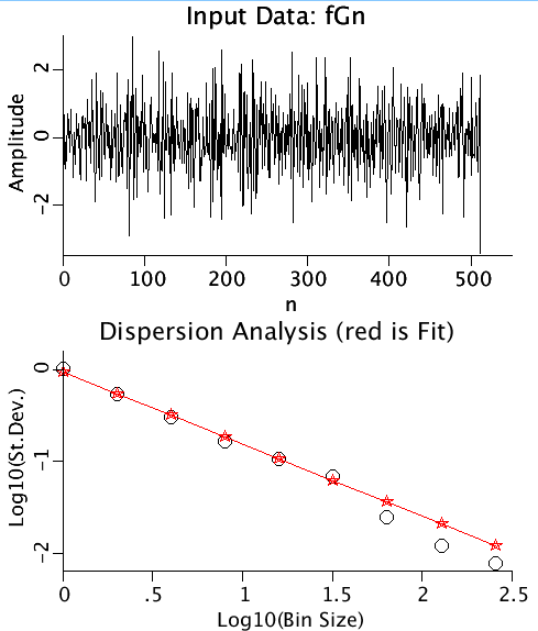
Upper Panel: A time series of Gaussianly distributed random numbers with mean=0, variance=4.
Lower Panel: The autocovariance function (black) and the autocorrelation function (red) are plotted as functions of the lag.

Equations

See Description above.

The equations for this model may be viewed by running the JSim model applet and clicking on the Source tab at the bottom left of JSim's Run Time graphical user interface. The equations are written in JSim's Mathematical Modeling Language (MML). See the Introduction to MML and the MML Reference Manual. Additional documentation for MML can be found by using the search option at the Physiome home page.