CV loop nonpulsatile model ported from Rideout (ACSL program PF-NP). Also in MATLAB.

Further reading:     Rideout's section 4.6, pages 117-125. 

Description

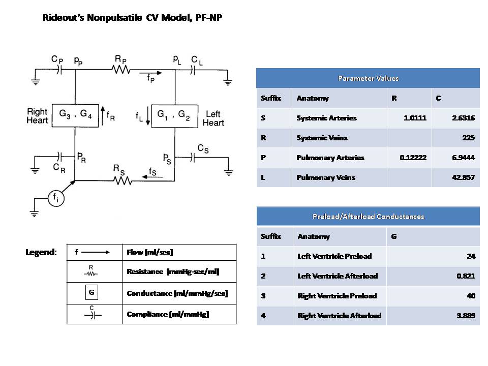
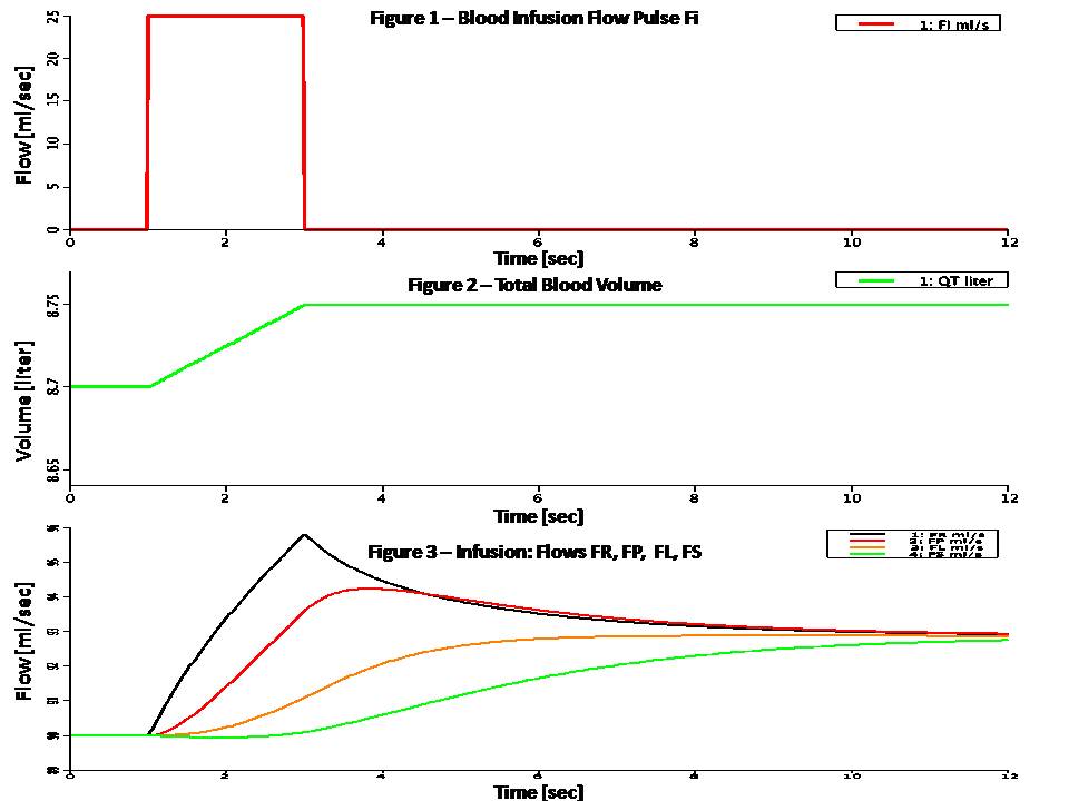
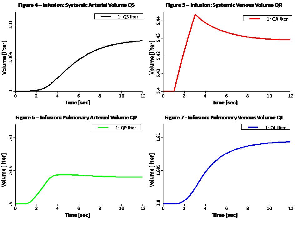
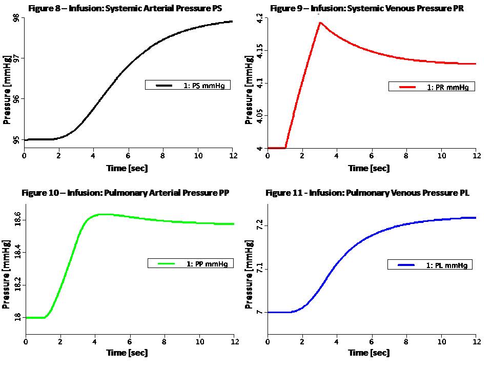
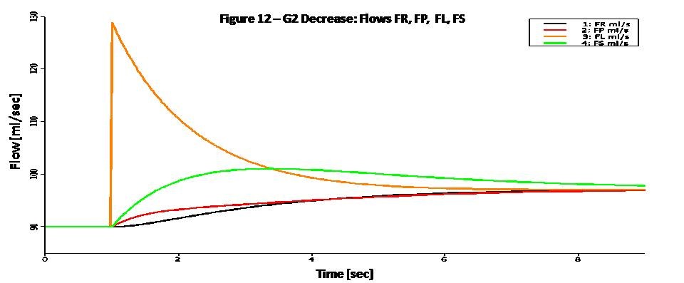
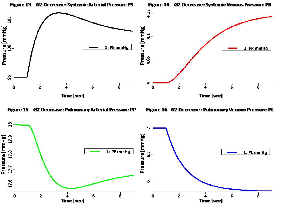
Nonpulsatile models are useful for pharmacokinetic studies which
typically have time constants in minutes. Ignoring nonlinearities, the
ventricular pressure-volume locus is counterclockwise between two
straight lines whose slopes are SD=1/CD and SS=1/CS. CD and CS are the
diastolic and maximum systolic compliances of the myocardium. If we
denote the end-diastolic pressure PED and end-systolic pressure PES,
then the stroke volume for the ventricle is:

QSV = PED * CD - PES * CS
									
Multiplying by the heart rate H, gives the average outflow:

F = (CD * H) * PED - (CS * H) * PES

Assuming a direct relationship between average atrial (Pat) pressure
and PED, and between average arterial (Part) pressure and PES, we get:

F = Gpre * Pat - Gafter * Part

Where Gpre and Gafter are the preload (prior to contraction) and
afterload (during ejection) conductances, and are inversely proportional
to the diastolic and systolic stiffness, respectively.

Denoting the left ventricle conductances G1 and G2, and the right
ventricle conductances G3 and G4, the following equations describe the
nonpulsatile ventricular flow:

FL = G1 * PL - G2 * PS
FR = G3 * PR - G4 * PP   (Eqs. 1)

The pressure drops over the systemic and pulmonary peripheral
resistances are given by Ohm's law:

PS - PR = RS * FS
PP - PL = RP * FP   (Eqs. 2)

Assuming fixed compliances and unstressed volume (under zero pressure)
for each of the four components:

PS = (QS - QSU) / CS
PR = (QR - QRU) / CR
PP = (QP - QPU) / CP
PL = (QL - QLU) / CL   (Eqs. 3)

Finally, integrating the flow through each component give the volume.
									
QS:t = FL - FS
QR:t = FS - FR + FI
QP:t = FR - FP
QL:t = FP - FL        (Eqs. 4)

Since this is a nonpulsatile model, the steady state is a unified
constant flow through the loop. It is interesting to model a sudden
change and the system response until a new steady state is obtained.
Two such conditions are modeled with a JSim choice variable:
(1) Infusion: Infusion flow pulse FI is added to systemic arteries
(2) Left Ventricular Stiffness Change: G2 is halved at time TCH

In infusion mode, a flow pulse FI is added to the systemic arteries
flow (second equation in Eqs. 4). The infusion pulse is rectangular,
starting at time TSTT = 1 sec and lasting WID = 2 seconds. In this
mode all conductances are fixed.

In Left Ventricular Stiffness Change mode, there is no infusion and
total blood volume is constant. Left ventricular afterload
conductance G2 is halved (left systolic stiffness is doubled) at
TCH = 1 sec.

Figure 1 shows the flow pulse FI in infusion mode. Figure 2 shows an
increase of 50 ml in total blood volume (integral of flow). Figure 3
shows the flows FR, FP, FL and FS in infusion mode. Figures 4 through 11
show the corresponding volumes and pressures.

Figure 12 shows the flows FR, FP, FL and FS in Left Ventricular
Stiffness Change mode. Figures 13 through 16 show the corresponding
pressures. The increase in systolic stiffness results in increased PS
and QS (as evident from Eqs. 3). PR and QR also increase, but somewhat
more slowly. As a result of these increases, the variables PP, QP, PL,
and QL decrease (total blood volume must remain constant). All flows
settle to the same increased value because of the stronger left heart.

Equations

The equations for this model may be viewed by running the JSim model applet and clicking on the Source tab at the bottom left of JSim's Run Time graphical user interface. The equations are written in JSim's Mathematical Modeling Language (MML). See the Introduction to MML and the MML Reference Manual. Additional documentation for MML can be found by using the search option at the Physiome home page.