Scaled Windowed Variance (SWV) Analysis for determining the Hurst coefficient from time series of fractional Brownian motion (fBm). Includes the linearly detrended (LDSWV) and bridge detrended (BDSWV) methods.

Description

This project contains the SWV (scaled Windowed Variance), LDSWV (Linearly
Detrended SWV), and BDSWV (Bridge Detrended SWV) algorithms as described
in Cannon, et. al (1997). These algorithms are designed to find the
value of the Hurst coefficient by analysing time series of fractional
Brownian motion (fBm).

A fBm time series of Length N is subdivided into bins of size 2^m where
m is an integer. In each bin the standard deviation is calculated. All
the data from the same size bins is averaged together. The slope of the 
logarithm of the averaged standard deviations as a function of the 
logarithm of the bin size is an estimate of the Hurst coefficient.

The input parameters to the model are
N               the number of data points in the input, were the x-values are
                the consecutive integers beginning with one.
PRETREAT        Choose  1   SWV Standard 8<=N<=511,
                        2 LDSWV Linearly detrended 512<=N<=2048, or
                        3 BDSWV Bridge detrended N>2049, depending on the
                          length of the series being analyzed.

EXCLUDE         If N is not 2^integer, then the binning of the data will
                leave a number excess points which is less than the bin size.
                Choose either end excess points ignored (the default) or
                front excess points ignored.

USE_BINS        Choose either default: Recommended bins or set bin sizes.
                Each algorithm has different recommended bin sizes. All
                bin sizes are given as log(actual bin size)/log(2).
                The default is documented in Cannon et al. (1997)
setBinStart     Used only if you are not using the recommended bin sizes.
                A value of 4 will give you a starting bin size of 16.
setBinEnd       Same directions as setBinStart. Should be greater than
                setBinStart.

SeeBinSize,     Allows user to see a subset of the data of size 2^SetBinSize
SeeBin          and a particular bin (1st, 2nd, Last). Values may be
                overridden if outside of range of algorithm.

The output variables are
Hurst           The Hurst coefficient describing the correlation of the fBm
                  (fractional Brownian motion) being analyzed.
AllSD           as a function of allBin. These are the binned standard deviations
                  as a function of bin size.
sd              as a function of binsize. These are the averaged standard 
                  deviations for each discrete binsize.
fit             as a function of binsize. This is the fit in log-log space 
                of sd(binsize).

input           is the data being analyzed as a function of point number.

locdata         is the data selected using the parameters SeeBinSize and SeeBin.
sub             what is being subtracted from this particular bin of data
                0 for SWV, the least squares fit line for LDSWV, or the line
                connecting the first and last points for this bin.
res             equals locdata minus sub. 

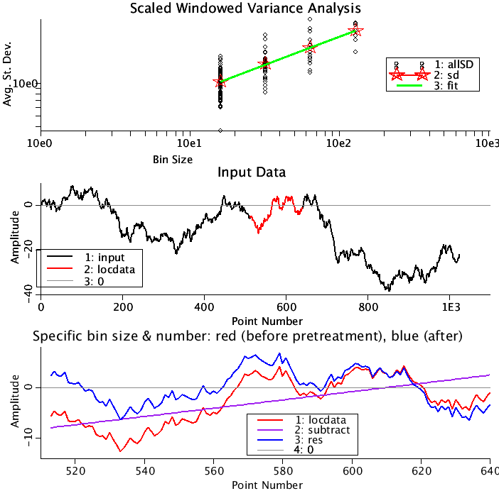
Upper Panel: All the calculated St. Deviations are plotted as a function of bin size (black circles). The averaged St. Deviations by bin size are plotted (red stars). The fit to the logarithms of the averaged St. Deviations vs. the logarithms of the bin size) is fit by a straight line(green). The slope of the green line is the estimate of the Hurst coefficient.
Middle Panel: The portion of the data being analyzed is plotted in black. (Note, N can be as large as 4096 for the fBm data set. The part of the series determined by the SeeBinSize and SeeBin is plotted in red.
Lower Panel: This is an enlargement of the data plotted in red in the middle panel. Here the data is plotted in red. What will be subtracted from this curve is plotted in purple. The result is plotted in blue. A thin gray line goes through zero. Run loops to see how the adjoining pieces connect.

Equations

See Description above.

The equations for this model may be viewed by running the JSim model applet and clicking on the Source tab at the bottom left of JSim's Run Time graphical user interface. The equations are written in JSim's Mathematical Modeling Language (MML). See the Introduction to MML and the MML Reference Manual. Additional documentation for MML can be found by using the search option at the Physiome home page.